
Micro and Macro Averaging#
Precision and Recall are two commonly used metrics to assess the performance of a classification model. The metrics are fairly intuitive with binary classification. But when it comes to multi-class classification these metrics need to be tweaked a bit to measure performance of each class.
This tutorial explains the concepts of micro and macro averaging and the scenarios in which to use each of the two approaches.
Basic Concepts#
Precision is the proportion of positive identifications that were actually correct.
Precision = \(\frac{True Positives}{True Positives + False Positives}\)
Recall is the proportion of the actual positives that were correctly identified.
Recall = \(\frac{True Positives}{True Positives + False Negatives}\)
Now let’s load some data and train a classifier.
from sklearn.datasets import load_iris as load_data, make_classification
from sklearn.ensemble import RandomForestClassifier
from sklearn.model_selection import train_test_split
from sklearn_evaluation import plot

X, y = load_data(return_X_y=True)

# split data into train and test
X_train, X_test, y_train, y_test = train_test_split(X, y, test_size=0.3, random_state=0)

y_pred = RandomForestClassifier(random_state=0).fit(X_train, y_train).predict(X_test)

target_names = ["A", "B", "C"]
Micro-average approach#
The micro-average precision and recall score is calculated from the individual classes’ true positives (TPs), true negatives (TNs), false positives (FPs), and false negatives (FNs) of the model. It aggregates the contributions of all classes to compute the average metric and weights each sample equally.
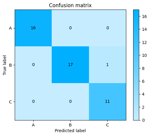
Let’s plot the confusion matrix and derive each metric.
plot.ConfusionMatrix.from_raw_data(y_test, y_pred, target_names=target_names)
<sklearn_evaluation.plot.classification.ConfusionMatrix at 0x7fa6ff02fe80>
Metrics for micro-average precision:
Note
True Positives (TPs) are the metrics on the main diagonal.
False Positives (FPs) are the metrics on the columns excluding the ones in the main diagonal, e.g., FPs for class A are cells (2,1) and (3,1).
\(TP_A\) = 16
\(FP_A\) = 0
\(TP_B\) = 17
\(FP_B\) = 0
\(TP_C\) = 11
\(FP_C\) = 1
Micro-average precision = \(\frac{TP_A + TP_B + TP_C} {TP_A + TP_B + TP_C + FP_A + FP_B + FP_C}\) = \(\frac{16+17+11} {16+17+11+0+0+1}\) = \(\frac{44}{45}\) = 0.97
Metrics for micro-average recall:
Note
False Negatives (FNs) are the metrics on the rows excluding the ones in the main diagonal, e.g., FNs for class A are cells (1,2) and (1,3).
\(FN_A\) = 0
\(FN_B\) = 1
\(FN_C\) = 0
Micro-average recall = \(\frac{TP_A + TP_B + TP_C} {TP_A + TP_B + TP_C + FN_A + FN_B + FN_C}\) = \(\frac{16+17+11} {16+17+11+0+1+0}\) = \(\frac{44}{45}\) = 0.97
We can see that the micro-average precision and micro-average recall values are the same. This is because, if there is false positive, there will always be a corresponding false negative and vice versa. For example, if a sample’s actual class is B, but it is predicted as A, it is a false positive for class A, but a false negative for class B.
Macro-average approach#
The macro-average precision and recall scores are calculated as arithmetic mean of individual classes’ precision and recall scores. Macro-average deals with aggregates or totals and studies the metrics as a whole.
Let’s view the classification report.
plot.ClassificationReport.from_raw_data(y_test, y_pred, target_names=target_names)
<sklearn_evaluation.plot.classification_report.ClassificationReport at 0x7fa6c5378e80>
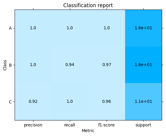
Macro-average precision = \(\frac{Precision_A + Precision_B + Precision_C} {3}\) = \(\frac{2.92}{3}\) = 0.97
Macro-average recall = \(\frac{Recall_A + Recall_B + Recall_C} {3}\) = \(\frac{2.94}{3}\) = 0.98
The Iris dataset used above is fairly balanced, and we can see in such cases the micro-average and macro-average precision and recall scores are the same.
Imbalanced Dataset#
Now let’s see how the micro and macro average scores vary when the dataset is an imbalanced one.
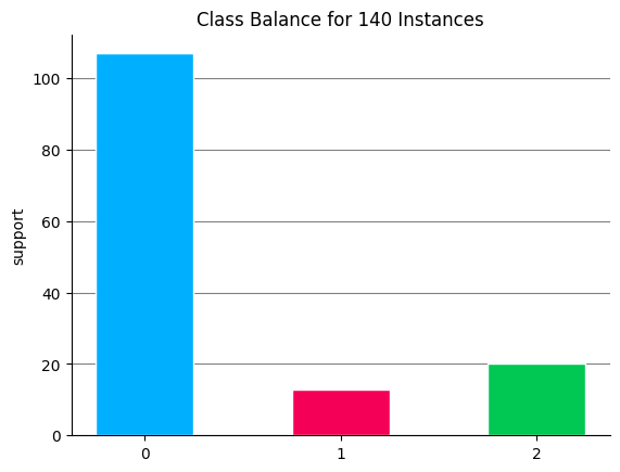
Let’s create an imbalanced dataset.
from sklearn.ensemble import RandomForestClassifier

X, y = make_classification(
    200,
    5,
    n_informative=3,
    n_classes=3,
    class_sep=0.8,
    weights=[0.75, 0.1, 0.15],
    random_state=0,
)

# split data into train and test
X_train, X_test, y_train, y_test = train_test_split(X, y, test_size=0.3, random_state=0)

y_pred = RandomForestClassifier(random_state=0).fit(X_train, y_train).predict(X_test)

target_names = ["A", "B", "C"]
plot.target_analysis(y_train)
<Axes: title={'center': 'Class Balance for 140 Instances'}, ylabel='support'>
Generate the metrics on this imbalanced dataset.
plot.ConfusionMatrix.from_raw_data(y_test, y_pred, target_names=target_names)
<sklearn_evaluation.plot.classification.ConfusionMatrix at 0x7fa6ff02f8e0>
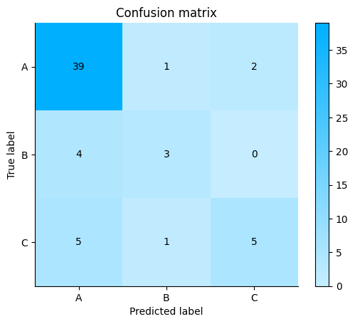
Micro-average precision = \(\frac{39+3+5}{39+3+5+9+2+2}\) = \(\frac{47}{60}\) = 0.78
Micro-average recall = \(\frac{39+3+5}{39+3+5+3+4+6}\) = \(\frac{47}{60}\) = 0.78
plot.ClassificationReport.from_raw_data(y_test, y_pred, target_names=target_names)
<sklearn_evaluation.plot.classification_report.ClassificationReport at 0x7fa6c4f425c0>
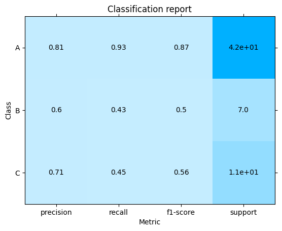
Macro-average precision = \(\frac {0.81 + 0.6 + 0.71} {3}\) = 0.70
Macro-average recall = \(\frac {0.93 + 0.43 + 0.45} {3}\) = 0.60
We can see that the macro-average precision and recall scores are lower than the micro-average ones. This is because the False Negatives of Classes B and C are higher than that of class A due to class imbalance.
Micro-average vs Macro-average#
If the dataset is balanced, both micro-average and macro-average will result in similar scores.
If the larger class in an imbalanced dataset performs better than the minority classes (the number of True Positives is significantly higher than the number of False Positives), the micro-average score will be higher than the macro-average score.
In a noisy dataset, the number of True Positives might be significantly lower than the number of False Positives for the majority class. In such a case, the macro-average score will be higher than the micro-average score. But this would be a bit misleading since a large number of examples are not properly classified.
Which approach to take#
Micro-averaging does not distinguish between classes and just averages the metrics. Hence, the scores are not affected if the test set is unequally distributed. Prefer this method if you are interested in the overall data and not inclined to a particular class.
If there is a class which occurs less frequently but is equally important as the rest, then macro-average is the preferred metric.
Tip
To understand how to plot micro-average curves, refer sklearn_evaluation.plot.ROC and sklearn_evaluation.plot.PrecisionRecall.